Basic Tutorial
[1]:
# Uncomment if PyGT has not been installed via pip
# import sys; sys.path.insert(0,"../")

import numpy as np
import matplotlib.pyplot as plt
# for colorbar placement
from mpl_toolkits.axes_grid1 import make_axes_locatable

# To construct rate matrix
from scipy.sparse import issparse, diags

import PyGT
Load in matrix and vectors selecting \(\mathcal{A,B}\) regions using the KTN format
KTN (Kinetic Transition Network) format requires two files:
min.datacolumns : \(E,\,2S/{\rm k_B},\,D,\,I_x,\,I_y,\,I_z\)
ts.datacolumns : \(E,\,2S/{\rm k_B},\,D,\,f,\,i,\,I_x,\,I_y,\,I_z\)
where
- \(E\) = Energy
- \(S\) = Entropy
- \(D\) = Degeneracy
- \(I_x\) = \(x\)-moment of intertia
- \(f,i\) = final,initial state indicies
Some technical details: - load_ktn() function looks for files [min,ts].data to build KTN, pruning isolated nodes, giving a new node indexing
load_ktn_AB()function looks for filesmin.[A,B]which use the same indicies as the data fileretainedis a vector that maps from the unpruned to pruned indexing convention, allowingmin.[A,B]to be read- Note that
A_vec, B_veccan clearly be determined without usingload_ktn_AB()orretained
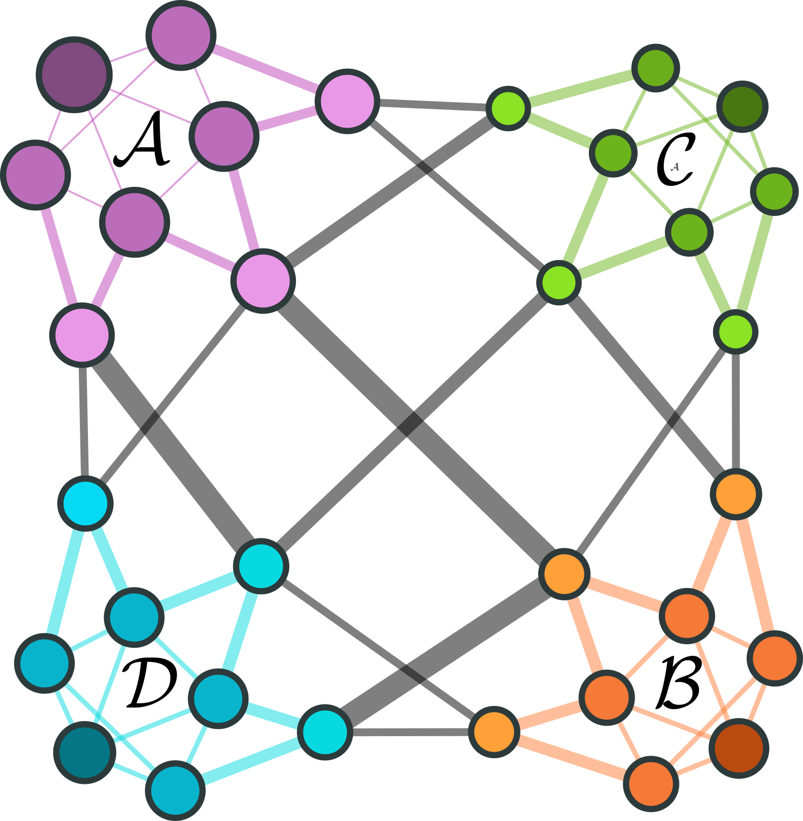
For this example we are loading in a 32 state network:
[1]:
from IPython.display import Image
Image(filename = "32state.png", width = 300)
[1]:
[2]:
data_path = "KTN_data/32state"
temp = 1.
beta = 1./temp

B, K, tau, N, u, s, Emin, retained = PyGT.io.load_ktn(path=data_path,beta=beta,screen=True)

F = u - s/beta # free energy

pi = np.exp(-beta * F) / np.exp(-beta * F).sum() # stationary distribution

# K has no diagonal entries
if issparse(K):
    Q = K - diags(1.0/tau)
else:
    Q = K - np.diag(1.0/tau)

A_vec, B_vec = PyGT.io.load_ktn_AB(data_path,retained)
I_vec = ~(A_vec+B_vec)
print(f'States in A,I,B: {A_vec.sum(),I_vec.sum(),B_vec.sum()}')

communities = PyGT.io.read_communities(data_path+"/communities.dat",retained,screen=True)
print('\nCommunities file identifies %d macrostates' % len(communities.keys()))
        Connected Clusters: 1, of which 95% have <= 32 states
        Retaining largest cluster with 32 nodes

States in A,I,B: (8, 16, 8)
Community 0: 8
Community 1: 8
Community 2: 8
Community 3: 8

Communities file identifies 4 macrostates
Remove a set of nodes in \(\mathcal{I}\) using graph transformation
- We remove all nodes in \(\mathcal{I} = (\mathcal{A}\cup\mathcal{B})^\mathsf{c}\) above the 10th percentile in free energy
- See documentation of
PyGT.tools.choose_nodes_to_remove()for other options
[3]:
rm_vec = PyGT.tools.choose_nodes_to_remove(rm_region=I_vec,
                                              pi=pi,
                                              tau=tau,
                                              style="free_energy",
                                              percent_retained=10
                                             )


gt_B, gt_tau, gt_K = PyGT.GT.blockGT(rm_vec,B,tau,block=10,rates=True,screen=True)
GT BECAME DENSE AT N=32, density=0.136719
GT done in 0.038 seconds with 0 floating point corrections
Find full MFPT matrix
Calculate the \(32 \times 32\) matrix of inter-microstate mean first passage times using GT.
[4]:
tauM = PyGT.mfpt.full_MFPT_matrix(B,tau,screen=True)
plt.matshow(tauM)
[4]:
<matplotlib.image.AxesImage at 0x7fe991f72190>

Find communitity MFPT matrix via full MFPT calculation or metastability approx
Reduced Boltzmann is the same in both cases
[5]:
#exact weighted-MFPT matrix
c_pi, c_tauM = PyGT.mfpt.community_MFPT_matrix(communities,B,tau,pi,MS_approx=False,screen=True)
#approximate weighted-MFPT matrix
c_pi, c_tauM_approx = PyGT.mfpt.community_MFPT_matrix(communities,B,tau,pi,MS_approx=True,screen=True)
#stationary distribution of macrostates
print(c_pi)
print(c_tauM)
#alternatively, we can compute the weighted-MFPTs from a pre-specified full inter-microstate MFPT matrix
ktn = PyGT.tools.Analyze_KTN(data_path, K=Q.todense(), pi=pi, commdata='communities.dat')
c_tauM_ktn = ktn.get_intercommunity_weighted_MFPTs(tauM)
print(c_tauM_ktn)
[0.31641201 0.19191359 0.25727061 0.23440379]
[[  0.         463.4908166  524.60802635 707.2325798 ]
 [511.6322427    0.         675.54122209 435.79646546]
 [575.5277695  678.31953914   0.         547.48055353]
 [861.79173354 542.2141931  651.11996412   0.        ]]
[[  0.         463.4908166  524.60802635 707.2325798 ]
 [511.6322427    0.         675.54122209 435.79646546]
 [575.5277695  678.31953914   0.         547.48055353]
 [861.79173354 542.2141931  651.11996412   0.        ]]
Plot ratio of exact to approximate MFPT matrix
Diagonal entries will be set to zero in application, but here we set diagonal terms to unity to avoid errors when taking ratio.
[6]:
c_tauM += np.eye(c_pi.size) - np.diag(c_tauM) # i.e. remove diagonal and replace with 1
c_tauM_approx += np.eye(c_pi.size) - np.diag(c_tauM_approx) # i.e. remove diagonal and replace with 1

plt.figure(figsize=(6,6),dpi=100)
plt.title(r"Matrix of $(\mathcal{T}_{\rm approx}-\mathcal{T})\,/\,\mathcal{T}$")
ax = plt.gca()
im = ax.matshow((c_tauM_approx-c_tauM)/c_tauM)
divider = make_axes_locatable(ax)
cax = divider.append_axes("right", size="5%", pad=0.05)
plt.colorbar(im, cax=cax)
[6]:
<matplotlib.colorbar.Colorbar at 0x7fe991872b20>

First passage time distribution between \(\mathcal{A}\) and \(\mathcal{B}\)
[7]:
moments, pt = PyGT.stats.compute_passage_stats(A_vec,B_vec,pi,Q,dopdf=True,rt=np.logspace(-6,2,400))

fig,axs = plt.subplots(1,2,figsize=(12,4),dpi=100)

axs[0].loglog(pt[:,0],pt[:,1]/moments[0])
axs[0].set_title(r"$\mathcal{A}\leftarrow\mathcal{B}$")
axs[0].set_ylabel(r"$p_{\rm fpt}(t)$")
axs[0].set_xlabel(r"$t$")
axs[1].loglog(pt[:,2],pt[:,3]/moments[2])
axs[1].set_title(r"$\mathcal{B}\leftarrow\mathcal{A}$")
axs[1].set_xlabel(r"$t$")

print("MFPT A<-B : ",moments[0],np.sqrt(moments[1]))
print("MFPT B<-A : ",moments[2],np.sqrt(moments[3]))
MFPT A<-B :  664.5826837564705 878.2798938434962
MFPT B<-A :  585.7934067017948 777.2852968888889

MFPTs and Phenomenological Rate Constants
Compute the mean first passage time and rates between \(\mathcal{A}\) and \(\mathcal{B}\).
[8]:
invtemps = np.linspace(0.01, 40, 10)
data = np.zeros((4, len(invtemps)))
for i, beta in enumerate(invtemps):
    B, K, tau, N, u, s, Emin, retained = PyGT.io.load_ktn(path=data_path,beta=beta,screen=False)
    F = u - s/beta # free energy
    pi = np.exp(-beta * F) / np.exp(-beta * F).sum() # stationary distribution
    rates = PyGT.stats.compute_rates(A_vec, B_vec, B, tau, pi, fullGT=False, MFPTonly=False, screen=False)
    data[0,i] = rates['kFAB']
    data[1,i] = rates['kFBA']
    data[2,i] = rates['MFPTAB']
    data[3,i] = rates['MFPTBA']

fig, (ax, ax1) = plt.subplots(1,2, figsize=(12,4), dpi=100)
ax.plot(invtemps, data[0,:], '-o', label='$k^F_{\mathcal{A} \leftarrow \mathcal{B}}$')
ax.plot(invtemps, data[1,:], '-o', label='$k^F_{\mathcal{B} \leftarrow \mathcal{A}}$')
ax1.plot(invtemps, data[2,:], '-o', label='$\mathcal{T}_{\mathcal{A} \leftarrow \mathcal{B}}$')
ax1.plot(invtemps,  data[3,:], '-o', label='$\mathcal{T}_{\mathcal{B} \leftarrow \mathcal{A}}$')
ax.set_xlabel('$1/T$')
ax1.set_xlabel('$1/T$')
ax.set_ylabel('Rate')
ax1.set_ylabel('MFPT')
ax.legend()
ax1.legend()
ax.set_yscale('log')
ax1.set_yscale('log')
